The Dataset:
We have the following data from Racine et al (1986) via BDA3:
| Dose (log g/ml) | Number of Rats | Number of Deaths |
|---|---|---|
| -0.86 | 5 | 0 |
| -0.30 | 5 | 1 |
| -0.05 | 5 | 3 |
| 0.73 | 5 | 5 |
Imports
NumPyro
import jax
from jax import numpy as jnp

import numpyro
from numpyro import distributions as dist, infer
Plotting and data manipulation
import pandas as pd
import matplotlib.pyplot as plt
import arviz as az
import seaborn as sns
Load the data
dose = [-0.86, -0.30, -0.05, 0.73]
numDeaths = [0,1,3,5]
numAnimals = [5,5,5,5]

data = pd.DataFrame(
	{
	"dose": dose,
	"deaths": numDeaths,
	"animals": numAnimals
	}
)
Set Up The Model
We have counts of deaths, so we'll use a binomial likelihood:
Where is the number of animals in the th group, and is the probability of death in the th group. The probability of death should be a function of the dose, so we could model this as:
But we need the to be between 0 and 1, so we'll use a logit function to map the linear predictor to the probability scale:
A corresponding NumPyro model here is:
logistic = lambda x: 1 / (1 + jnp.exp(-x))

def logisticmodel(dose, animals, deaths):
	alpha = numpyro.sample("alpha", dist.Uniform(-100, 100))
	beta = numpyro.sample("beta", dist.Uniform(-100, 100))

	with numpyro.plate("data", len(dose)):
		numpyro.sample("obs",
						dist.Binomial(animals,
						              logistic(alpha + beta*dose)),
						obs = deaths)
Sampling
First, set up the sampler (we're using NUTS here, while BDA3 uses a grid approx over the likelihood):
sampler = infer.MCMC(
    sampler = infer.NUTS(logisticmodel),
    num_chains = 1,
    num_samples = 2000,
    num_warmup= 1000
)
Next, sample from the model:
sampler.run(
    jax.random.PRNGKey(1),
    dose = jnp.array(data.dose),
    animals = jnp.array(data.animals),
    deaths = jnp.array(data.deaths)
)

samples = sampler.get_samples()
Results
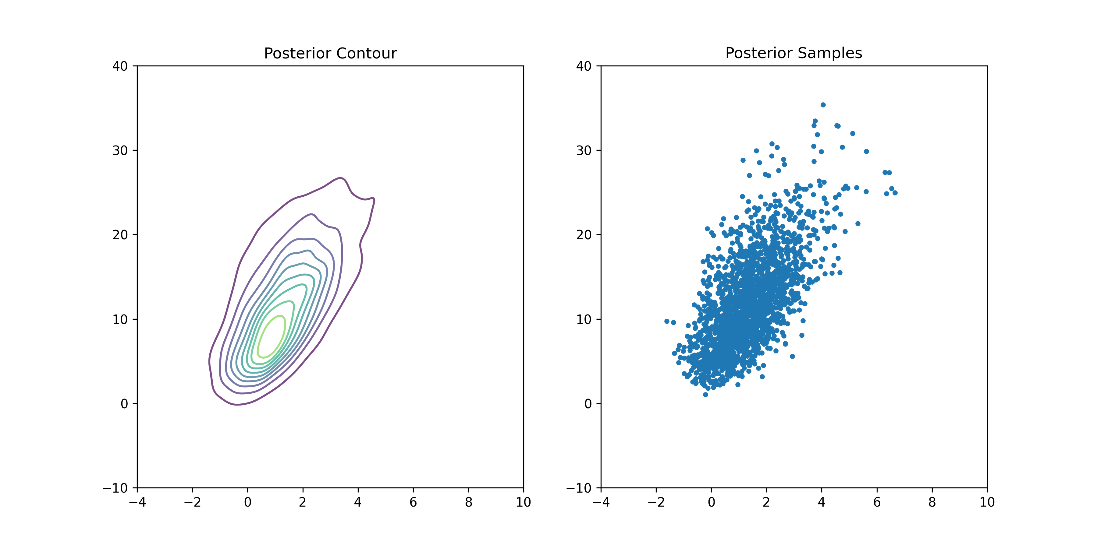
Posterior Analysis
We can reproduce Figure 3.3 from BDA:
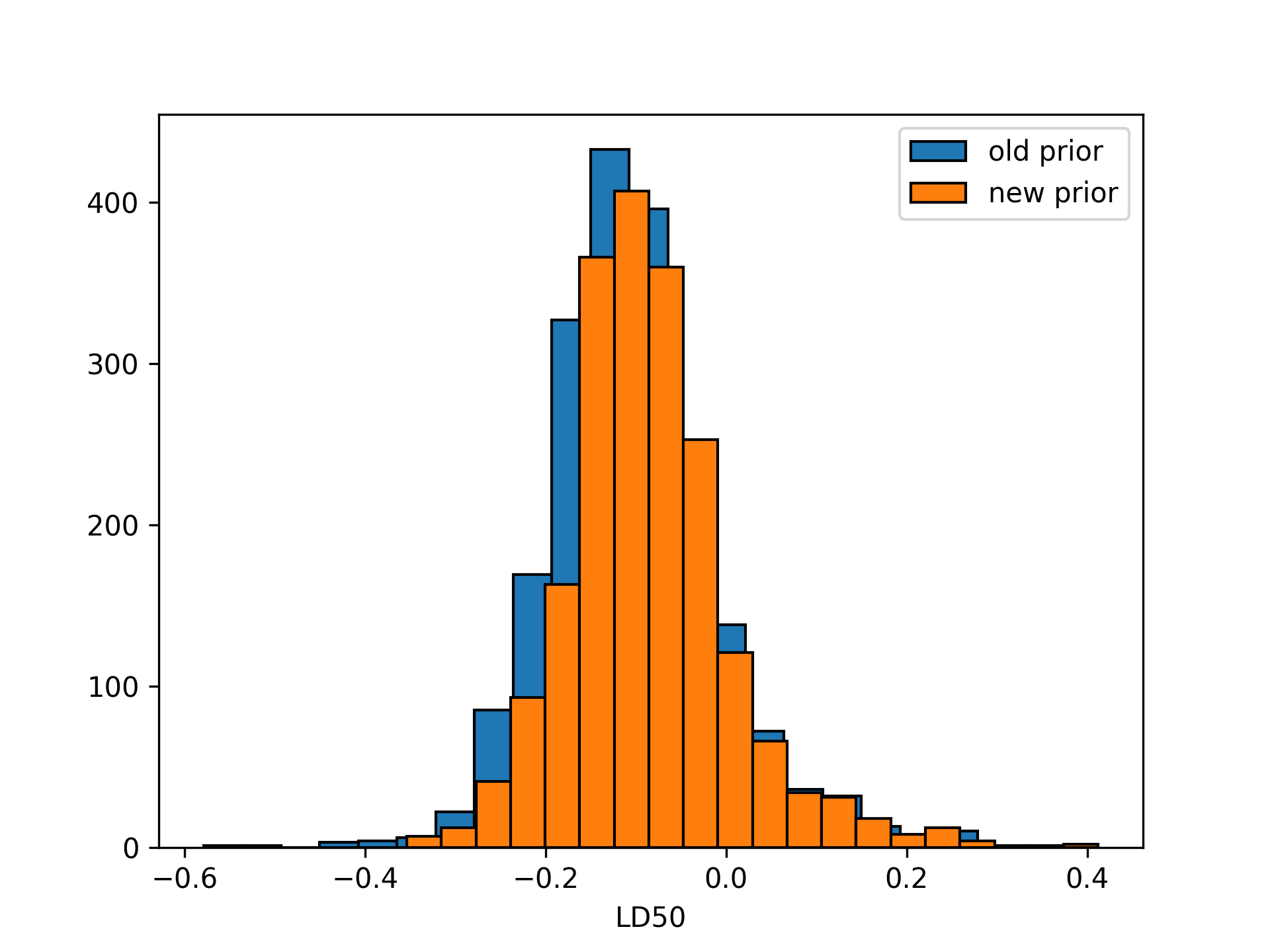
LD50 Distribution
What we want here is the dose () such that:
LD50 only makes sense if , so we'll restrict our attention to those samples:
# Posterior conditional on positive beta:
idx = samples["beta"] > 0
cond_samples = {k: v[idx] for k, v in samples.items()}

# Posterior LD50 distribution:
ld50_dist = cond_samples["alpha"] / -cond_samples["beta"]
Reproducing Figure 3.4 from BDA:
plt.hist(ld50_dist,
         bins = 20,
         color = "C0",
        edgecolor = "black")
plt.xlabel("LD50")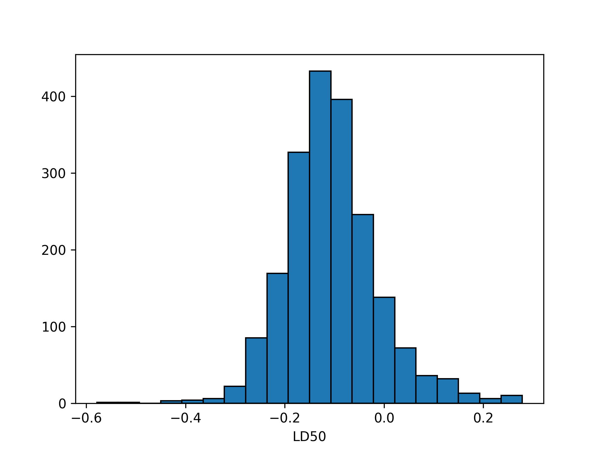
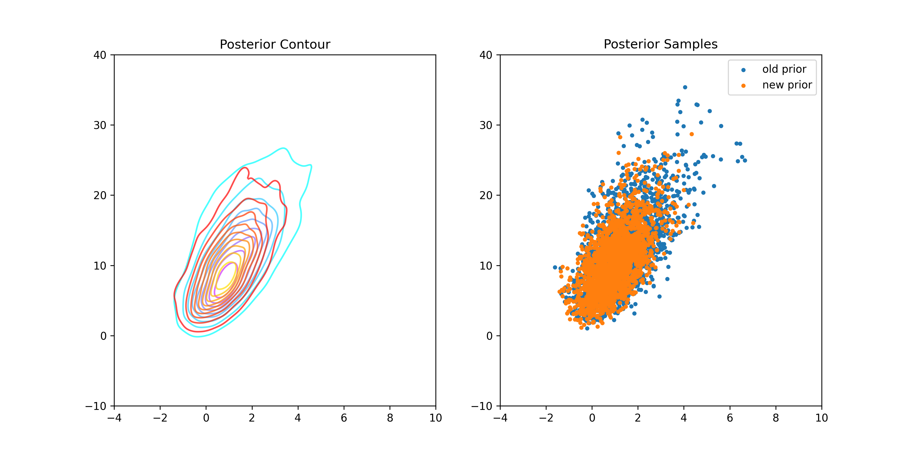
An Informative Prior:
BDA3 suggests a multivariate normal prior on and in one of the exercises.
BDA3 Pg. 82: Computation: in the bioassay example, replace the uniform prior density by a joint normal prior distribution on , with , , and
We can do the same in NumPyro:
def logisticmodel(dose, animals, deaths):
    mu = jnp.array([0, 10])
    cov_matrix = jnp.array([[2**2, 0.5 * 2 * 10],
                            [0.5 * 2 * 10, 10**2]])

    alpha, beta = numpyro.sample("alpha_beta",
                                 dist.MultivariateNormal(loc=mu,
                                    covariance_matrix=cov_matrix))

    with numpyro.plate("data", len(dose)):
        numpyro.sample("obs",
                       dist.Binomial(animals,
                                     logistic(alpha + beta*dose)),
                       obs = deaths)
Where inference proceeds exactly as before.
Parsing results:
NumPyro returns a dictionary of samples, where the keys are the strings in our numpyro.sample statements. We can put this back into the format of the original model:
alpha_samples = [float(val) for val,_ in samples["alpha_beta"]]
beta_samples =  [float(val) for _,val in samples["alpha_beta"]]

samples = {"alpha": alpha_samples,
           "beta": beta_samples}
Plotting the new posterior: