Imports:

Python:

import jax
import jax.numpy as jnp

import numpyro
from numpyro import distributions as dist, infer

import pandas as pd
import matplotlib.pyplot as plt
import arviz as az
import seaborn as sns

Data:

# BDA3 table 5.1 data: rat tumor
tumors = jnp.array([
    0,  0,  0,  0,  0,  0,  0,  0,  0,  0,  0,  0,  0,  0,  1,  1,  1,
    1,  1,  1,  1,  1,  2,  2,  2,  2,  2,  2,  2,  2,  2,  1,  5,  2,
    5,  3,  2,  7,  7,  3,  3,  2,  9, 10,  4,  4,  4,  4,  4,  4,  4,
    10,  4,  4,  4,  5, 11, 12,  5,  5,  6,  5,  6,  6,  6,  6, 16, 15,
    15,  9,  4
])
pop = jnp.array([
    20, 20, 20, 20, 20, 20, 20, 19, 19, 19, 19, 18, 18, 17, 20, 20, 20,
    20, 19, 19, 18, 18, 25, 24, 23, 20, 20, 20, 20, 20, 20, 10, 49, 19,
    46, 27, 17, 49, 47, 20, 20, 13, 48, 50, 20, 20, 20, 20, 20, 20, 20,
    48, 19, 19, 19, 22, 46, 49, 20, 20, 23, 19, 22, 20, 20, 20, 52, 46,
    47, 24, 14
])

Model:

The natural model here is a binomial model, with a beta prior on the probability of a tumours ($\theta$), so that we can exploit conjugacy if we want to. That is, we have the model:

In this case, we have prior information in the form of $70$ previous experiments which use the same variant of rat. In these experiments, we expect the latent probability of a tumour to vary according to the experiment – it is probably a function of environment, diet, and so on.

We denote these previous experiments as $(y_i, n_i)$, such that our current trial is $(y_{71}, n_{71})$, corresponding to the $(4, 14)$ scenario as originally outlined.

We can incorporate these other experiments into our model by estimating a unique $\theta_i$ for each experiment, with the values of $\theta_i$ drawn from a common prior over $\theta$ values. This extends the above model to:

We need to specify a hyperprior over $\alpha$ and $\beta$ –- BDA3 contains a long discussion on this issue. We choose to parametrize the mean and variance of the $\theta$ distribution, transforming to $\alpha$ and $\beta$ after sampling.

Our NumPyro model here is:

def rat_mod_full(y=None, n=None):
    # Hyperpriors
    mu = numpyro.sample("mu", dist.Beta(2, 2))
    tau = numpyro.sample("tau", dist.Gamma(2, 0.5))

    # Transformation to alpha, beta
    alpha = mu * tau
    beta = (1-mu) * tau

    # Prior on the probability of a tumour
    with numpyro.plate("theta_plate", len(pop)):
        theta = numpyro.sample("theta", dist.Beta(alpha, beta))

    # Likelihood
    with numpyro.plate("obs", len(pop)):
        numpyro.sample("y", dist.Binomial(n, theta), obs = y)

Inference:

We use NUTS to sample from the posterior:

sampler = infer.MCMC(
    infer.NUTS(rat_mod_full),
    num_warmup=500,
    num_samples=1000,
    num_chains=1,
)

sampler.run(
    jax.random.PRNGKey(1),
    y=jnp.array(tumors),
    n=pop
)

samples = sampler.get_samples()

Diagnostics:

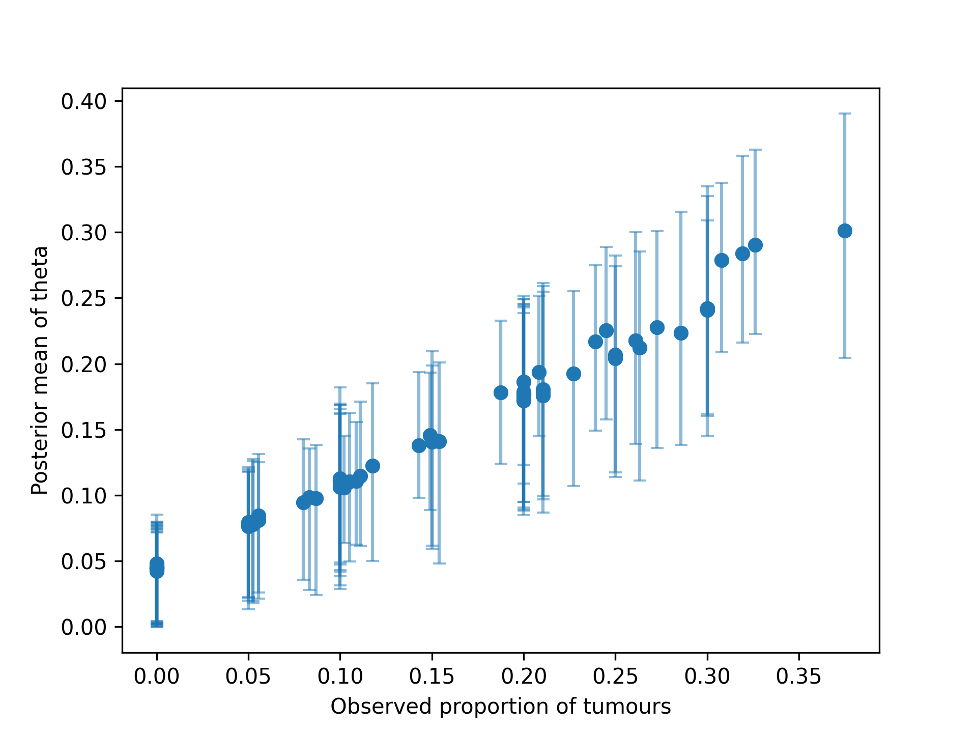
We can reproduce Figure 5.4 from BDA3: