Inference for Discrete Time Epidemic Models in Julia

The SIR model is a classic (maybe the classic) example of a compartment model in epidemiology. Compartment models treat epidemics as a series of flows between compartments:

Traditionally, the corresponding mathematical model is given as an ODE:

This approach has many benefits, especially with respect to inference. Unfortunately, these deterministic models can seriously underestimate uncertainty, especially when population sizes are small (see e.g. King et al 2015).

With this in mind, I'd like to get inference for a discrete, stochastic version of this model working in Julia. Again, unfortunately, inference for these models can be tricky:

1. The inclusion of discrete latent states makes inference with gradient based samples — e.g. HMC and NUTS — impossible (caveat: Li 2017, but I discuss this later).

2. The state space model here is non-linear and non-Gaussian, so the types of filtering methods we can use to compute pseudo-marginals (if we go that route) are restricted.

3. The parameter space itself –- e.g. the slice of the posterior composed of just ($\beta$, $\gamma$, prop_sus, init_inf, ...) can exhibit poor geometry for many MCMC samplers.

A Turing Model

Let's focus on (nearly) the simplest case of (nearly) the simplest model. We restrict our inference to just $\beta$ and the latent estimates, fixing $\gamma$ and \prop_rep to scalar values, and initial infections to one.

Making some data

@model function SIR(daily_inf, pop)
    # Parameters
    β ~ LogNormal(log(0.2), 0.02)
    γ = 0.1
    prop_rep = 0.8

    # Initialize States
    T = length(daily_inf)
    S = tzeros(T + 1)
    I = tzeros(T + 1)
    R = tzeros(T + 1)

    S[1] += pop - 1
    I[1] += 1
    
    infections = Vector{Int}(undef, T) # Allocate space for inferred infections
    recoveries = Vector{Int}(undef, T) # Allocate space for inferred recoveries
    
    # Process Simulation
    for t in 1:T
        infection_prob = -expm1(-β*I[t]/ (S[t] + I[t] + R[t]))
        recovery_prob = -expm1(-γ)
        
        infections[t] ~ Binomial(S[t], infection_prob)
        recoveries[t] ~ Binomial(I[t], recovery_prob)

        S[t+1] = S[t] - infections[t]
        I[t+1] = I[t] + infections[t] - recoveries[t]
        R[t+1] = R[t] + recoveries[t]

        # Likelihood of observed infections
        daily_inf[t] ~ Binomial(infections[t], prop_rep)
    end
end

We want some data to fit this to, and there's no nicer data than data from the prior!

model = SIR(zeros(100), 500) # 100 timesteps, 500 pop.
prior_chain = sample(model, Prior(), 100) # 100 prior samples

This gives us a chain with 1 + 2*len(dat) parameters –- Beta, and then latent infections (infections[t])) and recoveries (recoveries[t]). We'd like these infections and recoveries in a vector for plotting, so lets make a quick function to parse the chain into a nicer form:

function parse_chain(chain, index)
    s = DataFrame(chain)[index, :]
    inf_array = Vector(group(chain, :infections).value[index, :])
    rec_array = Vector(group(chain, :recoveries).value[index, :])

    return Dict(:β => s[:β],
                :infections => inf_array,
                :init_vector => [s[:β], inf_array..., rec_array...])
end

And finally, let's plot the data:

plot(data[:infections], theme = :wong2, legend = :false, alpha = :0.3);
scatter!(data[:infections], legend = :false, color = 1);
title!("Daily Infection Data")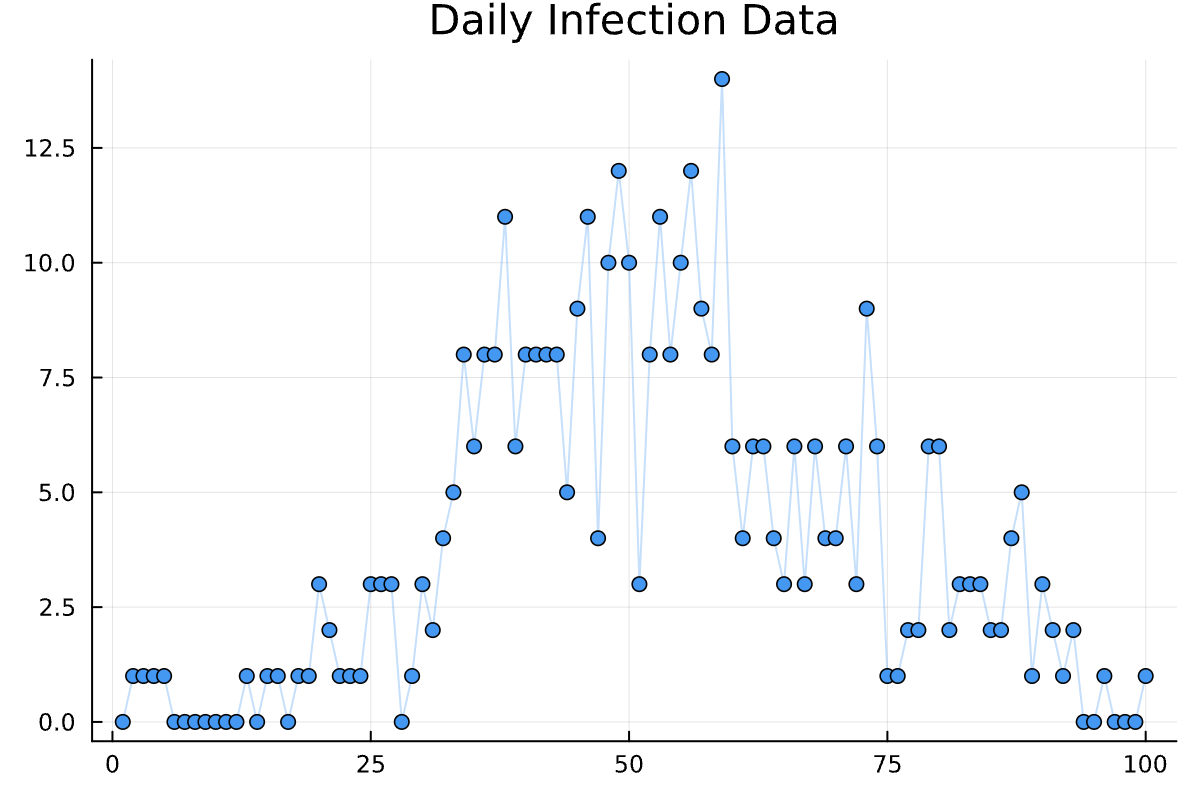

Sure, looks good.

Inference Attempt One

Ok, we have the model, we have the data — let's try conditioning the model on the data!